Step 1: Acquire the left and right views.
In this case, I got the left and right views directly from The Civil War, Part 3: The Stereographs. If you only have a scan of the stereocard, then you will have to use Gimp or Photoshop to get the left and right views, which is really quite easy.

Left view of stereocard.

Right view of stereocard.
If you are interested in who is actually seen in the picture, this is Alfred R. Waud, artist of Harper's Weekly, while he sketched on the battlefield near Gettysburg, Pennsylvania in July of 1863.
Step 2: Align the two views using ER9c.
The purpose of ER9c is to align the two views so that matches can be found later by the depth map generator along horizontal lines. As a side benefit, ER9c also gives you the minimum and maximum disparities which are needed by the depth map generator.
This is the input to ER9c:
image 1 (input) = main_1200_l.jpg
image 2 (input) = main_1200_r.jpg
rectified image 1 (output) = image_l.png
rectified image 2 (output) = image_r.png
Number of trials (good matches) = 10000
Max mean error (vertical disparity) = 10000
focal length = 1200
method = simplex
This is the output of ER9c (the important bits):
Mean vertical disparity error (before rectification) = 0.964856
Mean vertical disparity error = 0.410964
Min disp = -55 Max disp = 21
Min disp = -62 Max disp = 27
What you really want to see is a mean vertical disparity error after rectification (alignment) below 0.5. Of course, if it's below 1.0, it's ok too but not as good. The second line among the two that give min and max disparities gives you the min and max disparities to supply to the depth map generator.
The two rectified images are the ones to supply to the depth map generator.
As an alternative, one can also use ER9b but it is much more aggressive and the resulting two images may end up being heavily distorted. I cannot stress enough how important it is for the 2 views to be aligned/rectified before attempting to generate a depth map.
Step 3: Compute the depth map using DMAG5.
This is the input to DMAG5:
image 1 = ../image_l.png
image 2 = ../image_r.png
min disparity for image 1 = -62
max disparity for image 1 = 27
disparity map for image 1 = depthmap_l.png
disparity map for image 2 = depthmap_r.png
occluded pixel map for image 1 = occmap_l.png
occluded pixel map for image 2 = occmap_r.png
radius = 16
alpha = 0.9
truncation (color) = 30
truncation (gradient) = 10
epsilon = 255^2*10^-4
disparity tolerance = 0
radius to smooth occlusions = 9
sigma_space = 9
sigma_color = 25.5
downsampling factor = 2
As you can see, the minimum and max disparities come straight from the output of ER9c. The important bits here are the radius and the downsampling factor. The larger the images, the larger the radius should be. The downsampling factor speeds up the process at the possible expense of accuracy. Setting the downsampling factor to 2 cuts down the processing time by a factor of 4 when compared with setting the downsampling factor to 1 (no downsampling).

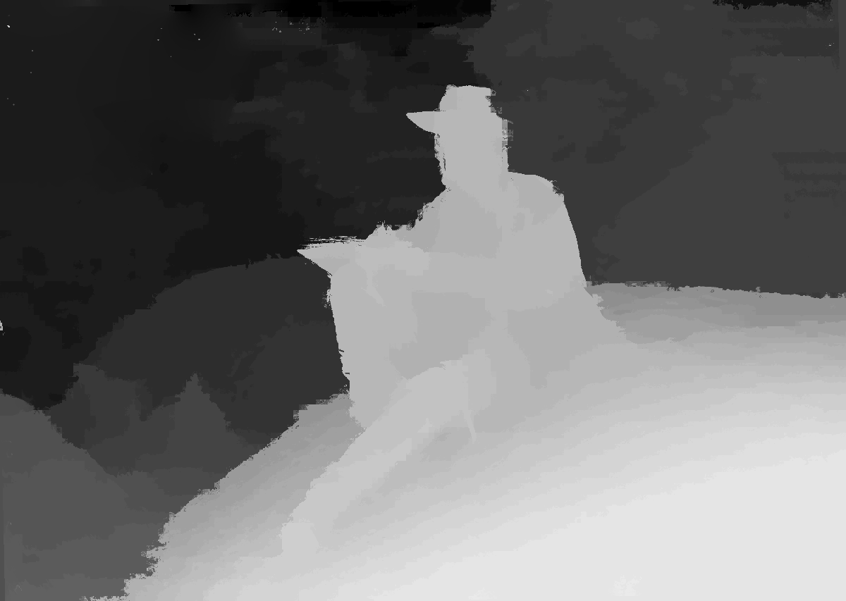
Depth map obtained by DMAG5.
Actually, that's pretty good right from the get go. In this particular case, I would skip the next step and go straight to step 5. Don't worry about the bad depths in the upper left corner as there is really nothing you can do about those unless you edit the depth map manually. We'll worry about those later.
If you want to see if you can get a better depth map from DMAG5, I would suggest changing the radius (try 8 and 32 and compare with 16). You may also want to change the downsampling factor from 2 to 1 but it's gonna take much longer to generate the depth map.
Step 4: Improve the depth map using DMAG9b.
I am doing this step to show how DMAG9b works. It is usually a good idea to try to improve the depth map using DMAG9b if the depth map is not so good near object boundaries. Here, you don't really need to bother as the depth map produced by DMAG5 is quite good. I am gonna show the process anyway as it's an important part of the pipeline for most stereo pairs.
This is the input to DMAG9b:
reference image = ../../image_l.png
input disparity map = ../depthmap_l.png
sample_rate_spatial = 32
sample_rate_range = 8
lambda = 0.25
hash_table_size = 100000
nbr of iterations (linear solver) = 25
sigma_gm = 1
nbr of iterations (irls) = 32
radius (confidence map) = 12
gamma proximity (confidence map) = 12
gamma color similarity (confidence map) = 12
sigma (confidence map) = 32
output depth map image = depthmap_l_dmag9b.png

It's a good start but we can certainly do better. The important bits are the spatial sample rate, the range (color) sample rate, and lambda. We are gonna play with those and see what happens.
Let's decrease the spatial sample rate from 32 to 16 without changing anything else.
This is the input to DMAG9b (the important bits):
sample_rate_spatial = 16
sample_rate_range = 8
lambda = 0.25

Better! Let's decrease the spatial sample rate from 16 to 8 without changing anything else.
This is the input to DMAG9b (the important bits):
sample_rate_spatial = 8
sample_rate_range = 8
lambda = 0.25

Even better! Let's stop messing around with the spatial sample rate and let's increase the range (color) sample rate from 8 to 16.
This is the input to DMAG9b (the important bits):
sample_rate_spatial = 8
sample_rate_range = 16
lambda = 0.25

Not a whole lot of difference. Let's go back and this time decrease the range (color) sample rate from 8 to 4.
This is the input to DMAG9b (the important bits):
sample_rate_spatial = 8
sample_rate_range = 4
lambda = 0.25

Again, not a whole lot of difference. Let's go back to a spatial sample rate of 8 and a range (color) sample rate of 8 and decrease lambda. The lambda parameter controls how smooth the depth is gonna be (in a joint-bilateral filtering sense where the joint image is the reference image). The larger lambda is, the smoother the depth is going to be. It sounds like a good thing but that's not always the case. If you don't want dmag9b to be too agressive and smooth too much, lambda should be lowered. If lambda is too large, you will see depths propagating along areas with similar color (in the reference image). The larger the spatial sample rate, the more you will notice depths propagating along areas of similar color.
This is the input to DMAG9b (the important bits):
sample_rate_spatial = 8
sample_rate_range = 8
lambda = 0.025

That's pretty good. Just for giggles, let's go the other way and increase lambda from 0.25 to 2.5.
This is the input to DMAG9b (the important bits):
sample_rate_spatial = 8
sample_rate_range = 8
lambda = 2.5

Yeah, that's not the direction you want to go. Let's stick to the depth map obtained using:
sample_rate_spatial = 8
sample_rate_range = 8
lambda = 0.025
Step 5: Edit the depth map using Gimp and DMAG11.
Up to now, I never really addressed the elephant in the room, the bad depths in the upper left corner. Well, here is the time to fix those and it's pretty easy using DMAG11. The input to DMAG11 is a reference image, that is, the left (rectified) image and a sparse depth map. Here, the sparse depth map is simply the current depth map where bad depth areas have been erased with the eraser tool in Gimp specifying hard edges, that is, with no anti-aliasing. When you start erasing the depth map, what you remove should turn to the checkerboard pattern. When you start erasing the depth map and it turns white, you need to first add an alpha channel to the depth map prior to erasing. To add an alpha channel, say to a jpeg depth map, you click on Layer->Transparency->Add Alpha Channel. When you save, save as png to preserve the alpha channel.

Sparse depth map. This is simply the depth map without the bad bits. Imagine that what's in white is actually a checkerboard pattern because that's how it actually looks (blogger always show transparent pixels as opaque white).
This is the input to DMAG11:
reference image = ../../../image_l.png
input depth map = ../sparse.png
output depth map = depth.png
radius = 4
gamma proximity = 10000
gamma color similarity = 2
maximum number iterations = 1000
scale number = 2
Output depth map from DMAG11.
Instead of using DMAG11, you can use DMAG4 with the same sparse depth map.
This is the input to DMAG4:
reference image = ../../../image_l.png
scribbled disparity map = ../sparse.png
edge image = ?
output disparity map = depth.png
beta = 90
maxiter = 10000
scale_nbr = 1
con_level = 1
con_level2 = 1

Output depth map from DMAG4.
I recommend using DMAG11 over DMAG4 unless you absolutely do not want depths to bleed over object boundaries. In this case, it is better to use DMAG4 with a so-called edge image. See Case Study - How to improve depth map quality with DMAG9b and DMAG4 for how to edit a depth map with DMAG4 using an edge image.
We are done with creating a decent depth map for our stereocard but let's go deeper into the rabbit hole.
Step 6: Create a wiggle/wobble with wigglemaker.
Before using wigglemaker, it is a good idea to crop and reduce the size of the reference image (the left image) and the final depth map.

Wobble created by wigglemaker.
The animation clearly show problems in the upper left corner and near/at the right side of his sketchbook. At this point, depending on how much of a perfectionist you are, you may want to go back to editing the depth map with Gimp (to erase the bad parts) and DMAG11 or DMAG4 (to fill in the blanks) to get an even better depth map. To fix the depth map on the right side of his sketchbook, I would use DMAG4 and an edge image. I might do that later.
Ok, I caved in and fixed the depth map using DMAG4 and an edge image. For the sparse depth map, I simply took the depth map and erased the little problems in the upper left corner and near the right side of his book. For the edge image, I simply traced along the area between foreground and background near the right side of his book.

Sparse depth map (white is really checkerboard pattern).

Edge image (white is really checkerboard pattern).
This is the input to dmag4:
reference image = ../../../../image_l.png
scribbled disparity map = sparse.png
edge image = edge.png
output disparity map = depth.png
beta = 10
maxiter = 10000
scale_nbr = 1
con_level = 1
con_level2 = 1

Output depth map obtained from DMAG4.
Because I am using an edge image, beta can be drastically lowered. If there is no edge image, I usually stick to 90 for beta but here I am using 10 for beta so that the depths can propagate very easily (unless they hit the edge image in which case they can't go across).

Wobble created with wigglemaker.
Of course, one could go crazy and trace en edge image all around the guy and erase the depth map all around the guy and apply DMAG4 to get close to a perfect depth map.


